lazy predict is a library that trains a large number of models on a given dataset to determine which one will work best for it
the goal is to predict a price range for a smartphone based on its specifications.
the specifcations include a total of 20 columns ranging from 3g availability to touch screen and amount of ram so a very extensive feature set.
import numpy as npimport pandas as pdimport matplotlib.pyplot as pltfrom matplotlib.pyplot import figureimport seaborn as snstrain = pd.read_csv("../input/mobile-price-classification/train.csv")test = pd.read_csv("../input/mobile-price-classification/test.csv")after loading in the data, lets take a look at it
train.head()| battery_power | blue | clock_speed | dual_sim | fc | four_g | int_memory | m_dep | mobile_wt | n_cores | ... | px_height | px_width | ram | sc_h | sc_w | talk_time | three_g | touch_screen | wifi | price_range | |
|---|---|---|---|---|---|---|---|---|---|---|---|---|---|---|---|---|---|---|---|---|---|
| 0 | 842 | 0 | 2.2 | 0 | 1 | 0 | 7 | 0.6 | 188 | 2 | ... | 20 | 756 | 2549 | 9 | 7 | 19 | 0 | 0 | 1 | 1 |
| 1 | 1021 | 1 | 0.5 | 1 | 0 | 1 | 53 | 0.7 | 136 | 3 | ... | 905 | 1988 | 2631 | 17 | 3 | 7 | 1 | 1 | 0 | 2 |
| 2 | 563 | 1 | 0.5 | 1 | 2 | 1 | 41 | 0.9 | 145 | 5 | ... | 1263 | 1716 | 2603 | 11 | 2 | 9 | 1 | 1 | 0 | 2 |
| 3 | 615 | 1 | 2.5 | 0 | 0 | 0 | 10 | 0.8 | 131 | 6 | ... | 1216 | 1786 | 2769 | 16 | 8 | 11 | 1 | 0 | 0 | 2 |
| 4 | 1821 | 1 | 1.2 | 0 | 13 | 1 | 44 | 0.6 | 141 | 2 | ... | 1208 | 1212 | 1411 | 8 | 2 | 15 | 1 | 1 | 0 | 1 |
5 rows × 21 columns
test.head()| id | battery_power | blue | clock_speed | dual_sim | fc | four_g | int_memory | m_dep | mobile_wt | ... | pc | px_height | px_width | ram | sc_h | sc_w | talk_time | three_g | touch_screen | wifi | |
|---|---|---|---|---|---|---|---|---|---|---|---|---|---|---|---|---|---|---|---|---|---|
| 0 | 1 | 1043 | 1 | 1.8 | 1 | 14 | 0 | 5 | 0.1 | 193 | ... | 16 | 226 | 1412 | 3476 | 12 | 7 | 2 | 0 | 1 | 0 |
| 1 | 2 | 841 | 1 | 0.5 | 1 | 4 | 1 | 61 | 0.8 | 191 | ... | 12 | 746 | 857 | 3895 | 6 | 0 | 7 | 1 | 0 | 0 |
| 2 | 3 | 1807 | 1 | 2.8 | 0 | 1 | 0 | 27 | 0.9 | 186 | ... | 4 | 1270 | 1366 | 2396 | 17 | 10 | 10 | 0 | 1 | 1 |
| 3 | 4 | 1546 | 0 | 0.5 | 1 | 18 | 1 | 25 | 0.5 | 96 | ... | 20 | 295 | 1752 | 3893 | 10 | 0 | 7 | 1 | 1 | 0 |
| 4 | 5 | 1434 | 0 | 1.4 | 0 | 11 | 1 | 49 | 0.5 | 108 | ... | 18 | 749 | 810 | 1773 | 15 | 8 | 7 | 1 | 0 | 1 |
5 rows × 21 columns
Data Analysis
# check data typestrain.info()<class 'pandas.core.frame.DataFrame'>RangeIndex: 2000 entries, 0 to 1999Data columns (total 21 columns): # Column Non-Null Count Dtype--- ------ -------------- ----- 0 battery_power 2000 non-null int64 1 blue 2000 non-null int64 2 clock_speed 2000 non-null float64 3 dual_sim 2000 non-null int64 4 fc 2000 non-null int64 5 four_g 2000 non-null int64 6 int_memory 2000 non-null int64 7 m_dep 2000 non-null float64 8 mobile_wt 2000 non-null int64 9 n_cores 2000 non-null int64 10 pc 2000 non-null int64 11 px_height 2000 non-null int64 12 px_width 2000 non-null int64 13 ram 2000 non-null int64 14 sc_h 2000 non-null int64 15 sc_w 2000 non-null int64 16 talk_time 2000 non-null int64 17 three_g 2000 non-null int64 18 touch_screen 2000 non-null int64 19 wifi 2000 non-null int64 20 price_range 2000 non-null int64dtypes: float64(2), int64(19)memory usage: 328.2 KB# check if there are any null columnstrain.isna().sum()battery_power 0blue 0clock_speed 0dual_sim 0fc 0four_g 0int_memory 0m_dep 0mobile_wt 0n_cores 0pc 0px_height 0px_width 0ram 0sc_h 0sc_w 0talk_time 0three_g 0touch_screen 0wifi 0price_range 0dtype: int64# describe the datatrain.describe()| battery_power | blue | clock_speed | dual_sim | fc | four_g | int_memory | m_dep | mobile_wt | n_cores | ... | px_height | px_width | ram | sc_h | sc_w | talk_time | three_g | touch_screen | wifi | price_range | |
|---|---|---|---|---|---|---|---|---|---|---|---|---|---|---|---|---|---|---|---|---|---|
| count | 2000.000000 | 2000.0000 | 2000.000000 | 2000.000000 | 2000.000000 | 2000.000000 | 2000.000000 | 2000.000000 | 2000.000000 | 2000.000000 | ... | 2000.000000 | 2000.000000 | 2000.000000 | 2000.000000 | 2000.000000 | 2000.000000 | 2000.000000 | 2000.000000 | 2000.000000 | 2000.000000 |
| mean | 1238.518500 | 0.4950 | 1.522250 | 0.509500 | 4.309500 | 0.521500 | 32.046500 | 0.501750 | 140.249000 | 4.520500 | ... | 645.108000 | 1251.515500 | 2124.213000 | 12.306500 | 5.767000 | 11.011000 | 0.761500 | 0.503000 | 0.507000 | 1.500000 |
| std | 439.418206 | 0.5001 | 0.816004 | 0.500035 | 4.341444 | 0.499662 | 18.145715 | 0.288416 | 35.399655 | 2.287837 | ... | 443.780811 | 432.199447 | 1084.732044 | 4.213245 | 4.356398 | 5.463955 | 0.426273 | 0.500116 | 0.500076 | 1.118314 |
| min | 501.000000 | 0.0000 | 0.500000 | 0.000000 | 0.000000 | 0.000000 | 2.000000 | 0.100000 | 80.000000 | 1.000000 | ... | 0.000000 | 500.000000 | 256.000000 | 5.000000 | 0.000000 | 2.000000 | 0.000000 | 0.000000 | 0.000000 | 0.000000 |
| 25% | 851.750000 | 0.0000 | 0.700000 | 0.000000 | 1.000000 | 0.000000 | 16.000000 | 0.200000 | 109.000000 | 3.000000 | ... | 282.750000 | 874.750000 | 1207.500000 | 9.000000 | 2.000000 | 6.000000 | 1.000000 | 0.000000 | 0.000000 | 0.750000 |
| 50% | 1226.000000 | 0.0000 | 1.500000 | 1.000000 | 3.000000 | 1.000000 | 32.000000 | 0.500000 | 141.000000 | 4.000000 | ... | 564.000000 | 1247.000000 | 2146.500000 | 12.000000 | 5.000000 | 11.000000 | 1.000000 | 1.000000 | 1.000000 | 1.500000 |
| 75% | 1615.250000 | 1.0000 | 2.200000 | 1.000000 | 7.000000 | 1.000000 | 48.000000 | 0.800000 | 170.000000 | 7.000000 | ... | 947.250000 | 1633.000000 | 3064.500000 | 16.000000 | 9.000000 | 16.000000 | 1.000000 | 1.000000 | 1.000000 | 2.250000 |
| max | 1998.000000 | 1.0000 | 3.000000 | 1.000000 | 19.000000 | 1.000000 | 64.000000 | 1.000000 | 200.000000 | 8.000000 | ... | 1960.000000 | 1998.000000 | 3998.000000 | 19.000000 | 18.000000 | 20.000000 | 1.000000 | 1.000000 | 1.000000 | 3.000000 |
8 rows × 21 columns
Explortary Data Analaysis
# number of samples for each price rangefig, ax = plt.subplots(figsize = (10, 4))sns.countplot(x ='price_range', data=train)plt.xlabel("Class Label")plt.ylabel("Number of Samples")plt.show()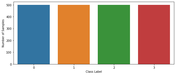
perfectly balanced, as all things should be.
# find correlationcorr_mat = train.corr()# each columns correlation with the pricecorr_mat['price_range']battery_power 0.200723blue 0.020573clock_speed -0.006606dual_sim 0.017444fc 0.021998four_g 0.014772int_memory 0.044435m_dep 0.000853mobile_wt -0.030302n_cores 0.004399pc 0.033599px_height 0.148858px_width 0.165818ram 0.917046sc_h 0.022986sc_w 0.038711talk_time 0.021859three_g 0.023611touch_screen -0.030411wifi 0.018785price_range 1.000000Name: price_range, dtype: float64# convert all to positive and sort by valueabs(corr_mat).sort_values(by=['price_range'])['price_range']m_dep 0.000853n_cores 0.004399clock_speed 0.006606four_g 0.014772dual_sim 0.017444wifi 0.018785blue 0.020573talk_time 0.021859fc 0.021998sc_h 0.022986three_g 0.023611mobile_wt 0.030302touch_screen 0.030411pc 0.033599sc_w 0.038711int_memory 0.044435px_height 0.148858px_width 0.165818battery_power 0.200723ram 0.917046price_range 1.000000Name: price_range, dtype: float64we can make a few observations from above
- the ram is the most deciding factor in price range with the highest correlation.
- the amount of pixels do matter after all.
- number of cores does not correlate with the price much (could be due to the cores being weak, for example most midrangers nowadays have 8 cores while the Apple A series SoCs have at most 6 cores and still perform miles better).
# battery correlation plotfig, ax = plt.subplots(figsize=(14,10))sns.boxenplot(x="price_range",y="battery_power", data=train,ax = ax)<matplotlib.axes._subplots.AxesSubplot at 0x7fa979ba8dd0>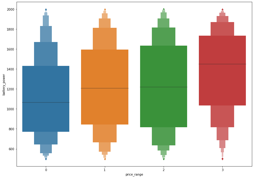
# individual correlation graphs# get all columns and remove price_rangecols = list(train.columns.values)cols.remove('price_range')# plot figurefig, ax = plt.subplots(7, 3, figsize=(15, 30))plt.subplots_adjust(left=0.1, bottom=0.05, top=1.0, wspace=0.3, hspace=0.2)for i, col in zip(range(len(cols)), cols): ax = plt.subplot(7,3,i+1) sns.lineplot(ax=ax,x='price_range', y=col, data=train)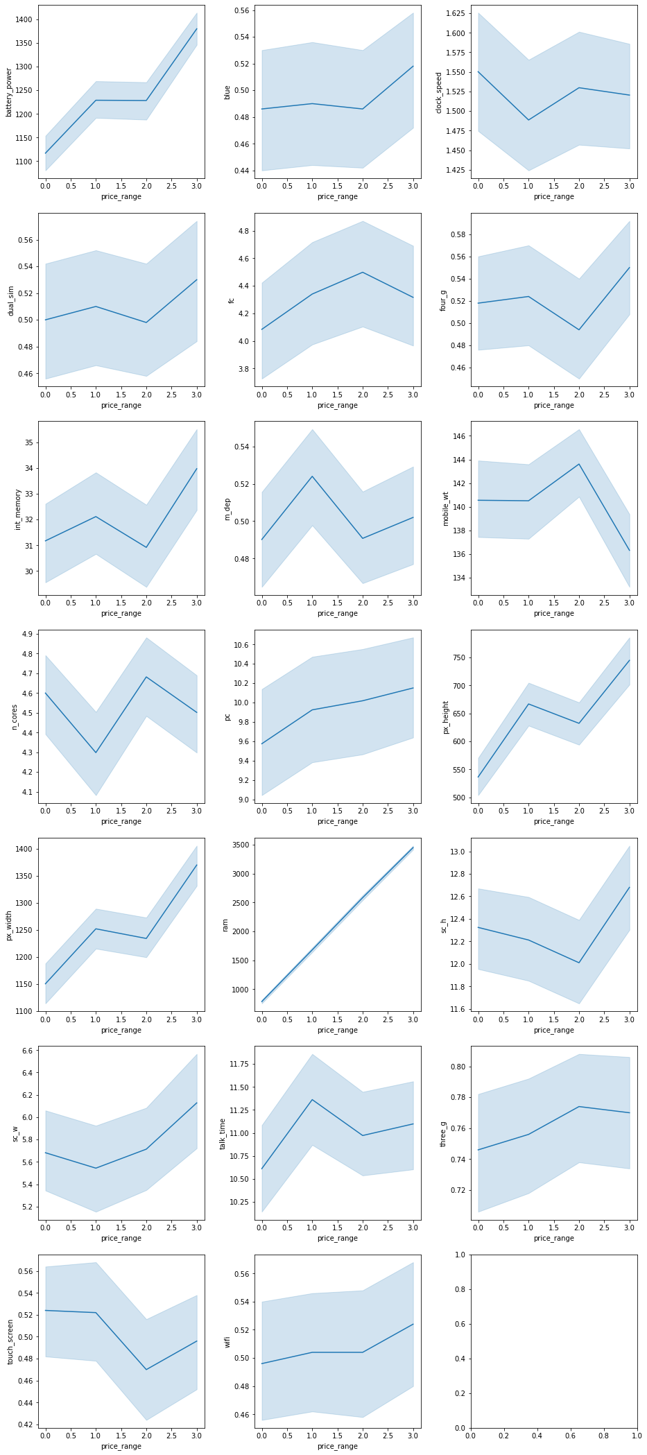
# plot full heatmapfigure(figsize=(20, 14))sns.heatmap(corr_mat, annot = True, fmt='.1g', cmap= 'coolwarm')<matplotlib.axes._subplots.AxesSubplot at 0x7fa9771fd850>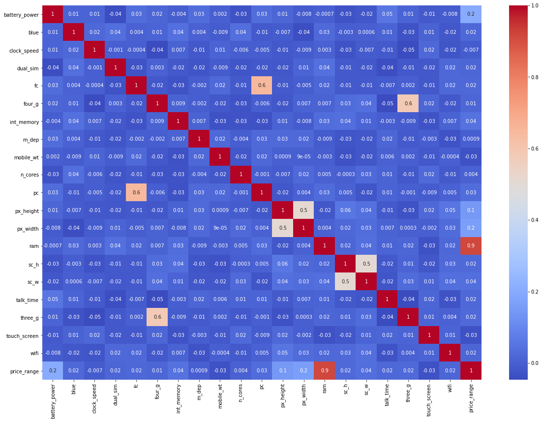
Modeling
knowing which model to build for a dataset is not an easy task, specially when the columns that have a high correlation with the target variable are less than half the total columns, its also a task that is time consuming in making and tuning these models that is why we will use the LazyPredict library to show us the results of various models without any tuneing and we will implement the top 3 models.
# extract target columntarget = train['price_range']# drop target column from datasettrain.drop('price_range', axis=1, inplace=True)from sklearn.model_selection import train_test_split# install and import lazypredict!pip install lazypredictfrom lazypredict.Supervised import LazyClassifier# split training dataset to training and testingX_train, X_test, y_train, y_test = train_test_split(train, target,test_size=.3,random_state =123)# make Lazyclassifier model(s)lazy_clf = LazyClassifier(verbose=0, ignore_warnings=True, custom_metric=None)# fit model(s)models, predictions = lazy_clf.fit(X_train, X_test, y_train, y_test)Requirement already satisfied: lazypredict in /opt/conda/lib/python3.7/site-packages (0.2.7)Requirement already satisfied: Click>=7.0 in /opt/conda/lib/python3.7/site-packages (from lazypredict) (7.1.1)[33mWARNING: You are using pip version 20.3.1; however, version 20.3.3 is available.You should consider upgrading via the '/opt/conda/bin/python3.7 -m pip install --upgrade pip' command.[0m100%|██████████| 30/30 [00:04<00:00, 6.21it/s]models| Accuracy | Balanced Accuracy | ROC AUC | F1 Score | Time Taken | |
|---|---|---|---|---|---|
| Model | |||||
| LogisticRegression | 0.94 | 0.95 | None | 0.94 | 0.06 |
| LinearDiscriminantAnalysis | 0.93 | 0.93 | None | 0.93 | 0.07 |
| QuadraticDiscriminantAnalysis | 0.92 | 0.92 | None | 0.92 | 0.02 |
| LGBMClassifier | 0.91 | 0.91 | None | 0.91 | 0.48 |
| XGBClassifier | 0.91 | 0.91 | None | 0.90 | 0.41 |
| RandomForestClassifier | 0.87 | 0.87 | None | 0.87 | 0.50 |
| SVC | 0.86 | 0.87 | None | 0.86 | 0.17 |
| NuSVC | 0.86 | 0.87 | None | 0.86 | 0.22 |
| BaggingClassifier | 0.86 | 0.87 | None | 0.86 | 0.13 |
| ExtraTreesClassifier | 0.84 | 0.85 | None | 0.84 | 0.37 |
| DecisionTreeClassifier | 0.84 | 0.84 | None | 0.84 | 0.03 |
| LinearSVC | 0.82 | 0.83 | None | 0.82 | 0.32 |
| CalibratedClassifierCV | 0.81 | 0.82 | None | 0.80 | 1.06 |
| GaussianNB | 0.78 | 0.79 | None | 0.78 | 0.02 |
| PassiveAggressiveClassifier | 0.74 | 0.75 | None | 0.74 | 0.03 |
| SGDClassifier | 0.73 | 0.74 | None | 0.72 | 0.05 |
| Perceptron | 0.73 | 0.74 | None | 0.73 | 0.03 |
| NearestCentroid | 0.70 | 0.70 | None | 0.70 | 0.02 |
| AdaBoostClassifier | 0.63 | 0.62 | None | 0.61 | 0.22 |
| RidgeClassifier | 0.56 | 0.58 | None | 0.47 | 0.04 |
| RidgeClassifierCV | 0.56 | 0.58 | None | 0.47 | 0.02 |
| BernoulliNB | 0.53 | 0.54 | None | 0.52 | 0.03 |
| KNeighborsClassifier | 0.52 | 0.52 | None | 0.52 | 0.08 |
| ExtraTreeClassifier | 0.51 | 0.51 | None | 0.51 | 0.02 |
| LabelSpreading | 0.45 | 0.45 | None | 0.45 | 0.20 |
| LabelPropagation | 0.45 | 0.45 | None | 0.45 | 0.15 |
| DummyClassifier | 0.26 | 0.26 | None | 0.26 | 0.02 |
| CheckingClassifier | 0.25 | 0.25 | None | 0.10 | 0.02 |
# plot the first 5 models F1 scoretop = models[:5]figure(figsize=(14, 7))sns.lineplot(x=top.index, y="F1 Score", data=top)<matplotlib.axes._subplots.AxesSubplot at 0x7fa946d44bd0>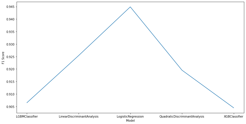
we are not really intrested in the predictions dataframe here because we already know those values and they’re part of the training dataset
from above we can see that the best algorithm for this type of task is logistic regression followed by Discriminant Analysis models and followed closely by GB models.
Implemented models
- logistic regression
- Linear Discriminant Analysis
- light GBM classifier
the reason behing skipping on the Quadratic Discriminant Analysis model is because its of the same family as Linear Discriminant Analysis and produces similar results, we also want to implement a diverse range of models
from sklearn.linear_model import LogisticRegression# Logistic regressionlog_clf = LogisticRegression(random_state=0).fit(train, target)# drop the id column from test to match the size of traintest.drop('id', axis=1, inplace=True)# get predictions on test dataset and convert it to a dataframelog_preds = pd.DataFrame(log_clf.predict(test), columns = ['log_price_range'])log_preds.head()| log_price_range | |
|---|---|
| 0 | 2 |
| 1 | 3 |
| 2 | 2 |
| 3 | 3 |
| 4 | 2 |
from sklearn.discriminant_analysis import LinearDiscriminantAnalysis# Linear Discriminant Analysislda_clf = LinearDiscriminantAnalysis().fit(train, target)# get predictions on test dataset and convert it to a dataframelda_preds = pd.DataFrame(lda_clf.predict(test), columns = ['lda_price_range'])lda_preds.head()| lda_price_range | |
|---|---|
| 0 | 3 |
| 1 | 3 |
| 2 | 2 |
| 3 | 3 |
| 4 | 1 |
from lightgbm import LGBMClassifier# lightgbm modellgbm_clf = LGBMClassifier(objective='multiclass', random_state=5).fit(train, target)# get predictions on test dataset and convert it to a dataframelgbm_preds = pd.DataFrame(lgbm_clf.predict(test), columns = ['lgbm_price_range'])lgbm_preds.head()| lgbm_price_range | |
|---|---|
| 0 | 3 |
| 1 | 3 |
| 2 | 3 |
| 3 | 3 |
| 4 | 1 |
comparing model results
# create dataframe with 3 columns and index from any of the predicted dataframesresults = pd.DataFrame(index=log_preds.index, columns=['log', 'lda', 'lgbm'])# add in data from the 3 predicted dfsresults['log'] = log_predsresults['lda'] = lda_predsresults['lgbm'] = lgbm_preds# show grouped dfresults| log | lda | lgbm | |
|---|---|---|---|
| 0 | 2 | 3 | 3 |
| 1 | 3 | 3 | 3 |
| 2 | 2 | 2 | 3 |
| 3 | 3 | 3 | 3 |
| 4 | 2 | 1 | 1 |
| ... | ... | ... | ... |
| 995 | 1 | 2 | 2 |
| 996 | 1 | 1 | 1 |
| 997 | 2 | 0 | 0 |
| 998 | 1 | 2 | 2 |
| 999 | 3 | 2 | 2 |
1000 rows × 3 columns
# find columns where all 3 models agree on the resultequal_rows = 0for row in results.itertuples(index=False): if(row.log == row.lda == row.lgbm): equal_rows += 1equal_rows628from all the 1000 rows the 3 models agree on 62% which means any of these 3 algorithms should be n overall good choice for predicting the price range of a smartphone based on its specifications